COS 513 Project

Team: Lydia Liu, Niranjani Prasad, Kiran Vodrahalli

More Results on EEG-fMRI

First of all, we decided to tackle the EEG-fMRI problem again. However, one main difficulty with the dataset is shown in the following picture:

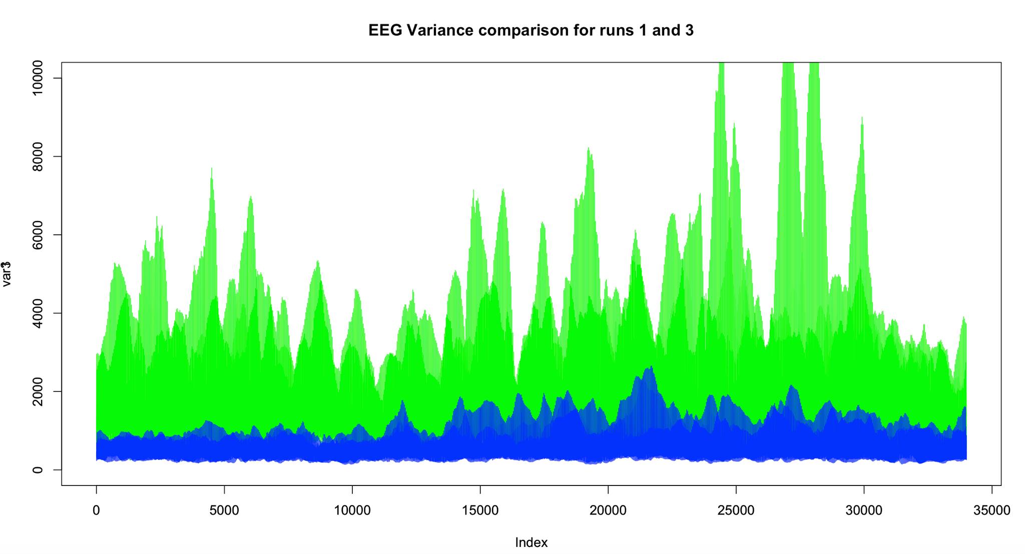
Across trials, the data seems to behave very differently.

Here is a summary of the results.

Change of Direction: Predicting MEG response from an image

To summarize the new learning problem, we have \(92\) pairs of MEG-image data. The MEG has \(306\) channels; each channel has a \(k\)-dim frequency vector which has as entries the coefficients of FFT on the time series data for the channel. We select \(k\). We will represent the image in two ways:

• Naive version: grayscale image vector
• Convolutional neural network layer features stacked on top of each other in a vector format. We get the CNN as a pre-trained model on the large ImageNet dataset (using Caffe from Berkeley Vision).

For each of the \(306\) channels we learn a matrix: \(F = AL\) where \(F\) is the \(k \times 92\) matrix of frequency vectors for the given channel for each of the \(92\) pairs; L is the \(m \times 92\) matrix of image vectors for each of the \(92\) pairs, and \(A\) is \(k \times m\) matrix that we learn for each of the \(306\) channels. Then, putting all \(306\) channels together, we get a tensor ((T)) which is \(306 \times k \times m\).We learn each of these matrices separately with ridge regression (to ensure we get a unique solution for each problem).

We get frequency vectors by taking FFT of each of the MEG time series and using \(k\) of the resulting coefficients. For each individual, we have \(42\) examples of the individual looking at the same picture, and we have \(15-20\) individuals. We average separately for each channel to get the \(306\) frequency vectors for a given image.

Now we present in more detail how to get the image representations. In the naive case, we just use the grayscale image in \((175 * 175) \times 1\) vector format. In the case of using convolutional neural networks, we use a known convolution net that works well (GoogLeNet), and run each of the \(92\) object images through the convolutional net to produce the outputs at each layer. From here, we vectorize each of the layer outputs and stack each layer on top of the others (making sure that the layer entries are adjacent) so that we have a long thin vector. We can choose to use only features from a single layer of the net, or we can use multiple layers to build our vector. Then, note that the \(k \times m\) matrix that we learn will have a \(k \times l^{(i)}\) matrix for each layer feature \(i\), where \(l^{(i)}\) is the number of pixels in feature layer \(i\).

The overall outline is summarized in the following diagram:

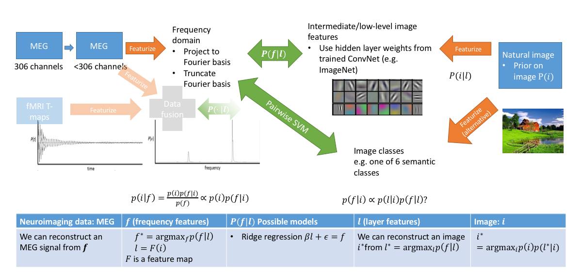
We can also potentially featurize our image with a probability vector, where probability is taken over feature layers. Then if we have a generative model for feature layers of our convolutional net, we get a generative model for MEG data. Moreover, given any MEG data, we can solve a simple convex optimization problem to get the probability vector, which we can then apply to generate an image representing a given MEG input. This would give us a generative model for MEG with an image prior!

Visualization

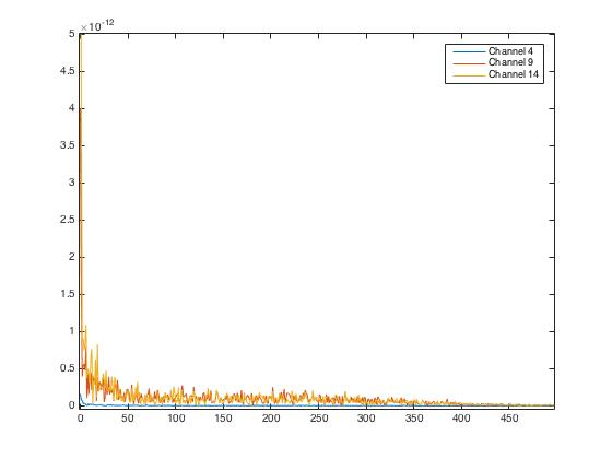
Here we plot the \(4^{th}, 9^{th}, 14^{th}\) channel MEG responses of the first individual, first trial for the first image:

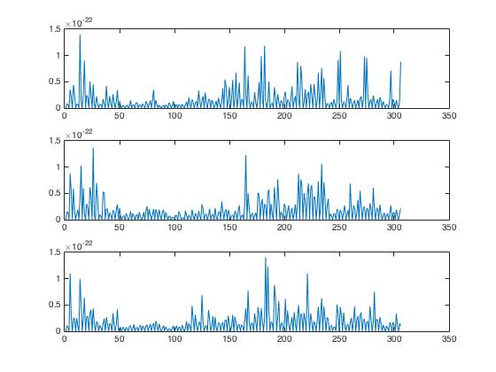
For \(3\) of the \(92\) image-MEG pairs, we plot the sum of the Fourier coefficients for each of the \(306\) channels of the MEG in order to get a rough idea of the activity associated with each MEG channel in response to the first three images. The MEG data is from one trial of the same person.

Naive Result

Ridge and LASSO regression using the basic image as input to predict the frequencies do not work well. We will try the convolutional network implementation next.

Preliminary Results from Sparse CCA

First of all, we did some more pre-processing steps and changed the format of the fMRI data to both account for potential lag in correlation between the EEG and fMRI as well as to introduce a time component into our representation of fMRI. We stacked three fMRI TRs together in a sliding window fashion. Thus, our pairs for sCCA are now (\(2000 \times 34\) EEG, \(3\) TRs of smoothed and downsampled fMRI).

Here we plot the vector pair (EEG, fMRI) of highest correlation. The correlation of the top vector is around \(0.83\). This is for the case where we ask for \(K = 20\) features from sCCA.

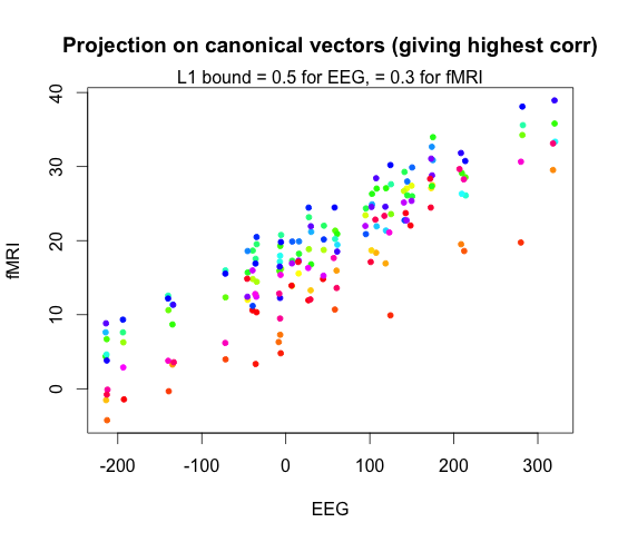
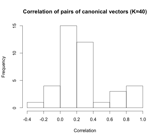
When we set \(K = 40\), this is what the highest correlation canonical vector plot looks like. The correlation was \(0.98\).

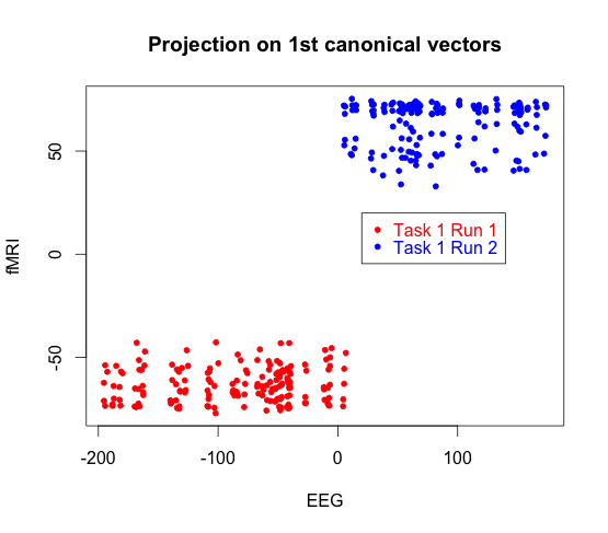
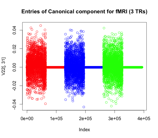
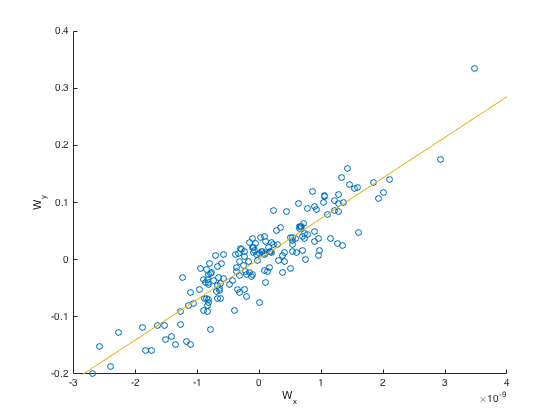
Here we display a canonical vector for EEG plotted again a canonical vector for fMRI. The red data points come from subject one task one run one, and the blue points come from subject two task two run two.

Here we give a histogram showing the number of vectors for each correlation level for \(K = 20\)

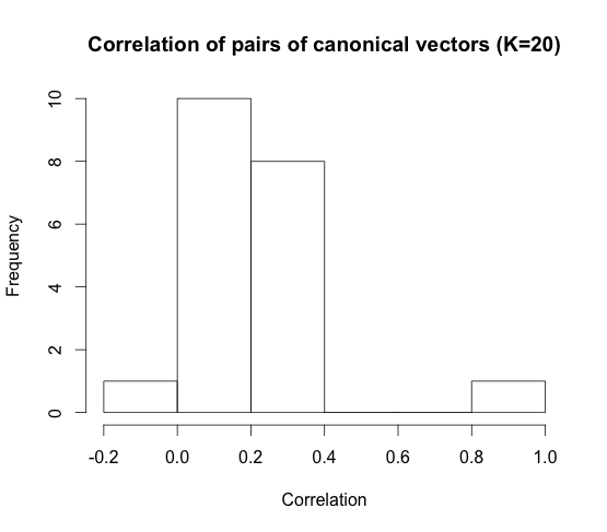
When we set \(K = 40\) features, these are what the correlation histogram looks like.

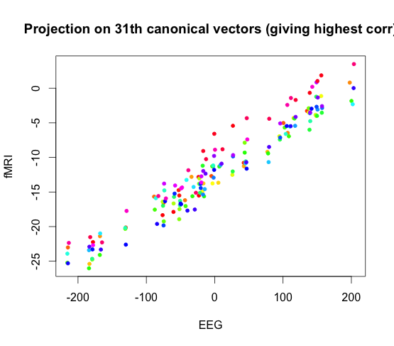
Here we plot for a single representation of fMRI (which consists of three TRs) what the canonical vector values look like.

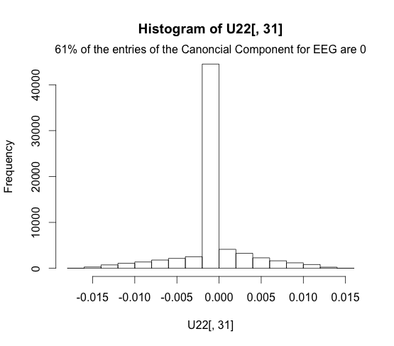
Here we plot the sparsity of the fMRI representation.

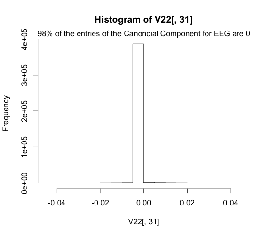
We can see that the EEG representation is a bit less sparse, due to the settings of the LASSO parameter.

Preliminary Analyses of the MEG-fMRI Dataset

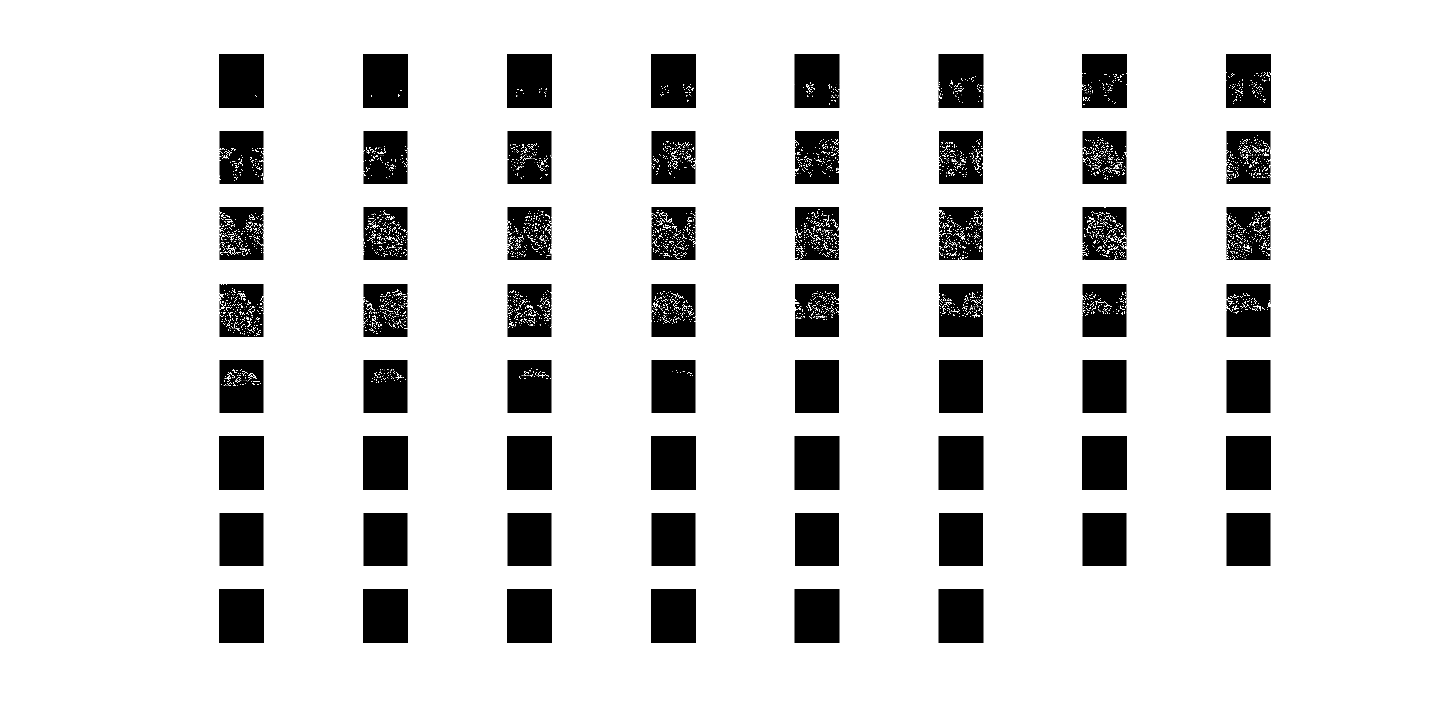
Here we visualize the \(t\)-map values from the MEG-fMRI dataset. The \(t\)-map was calculated by using a GLM to predict images based on the input of fMRI data. The GLM learned a weight for each voxel: Here we have displayed that weighting for one subject and one image class.

Then we decided to run sparseCCA on the MEG-fMRI data as well with \(K = 20\).

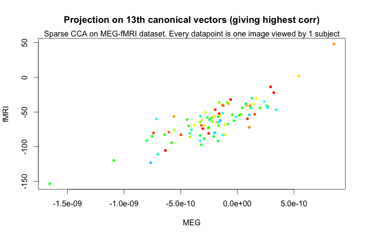
Here we plot the projections onto the highest correlation canonical vectors for MEG and fMRI-t-values. The correlation was \(0.84\).

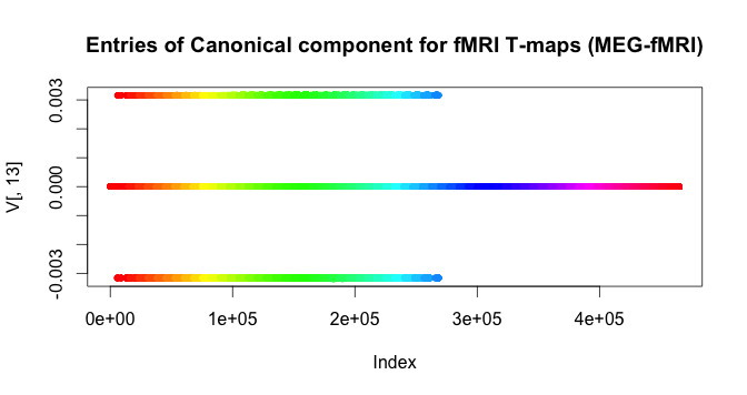
Here we visualize the values of the highest correlation canonical vector for the fMRI-t-values.

Ideas about Generative Models

For a naive approach to start out with, we were considering simply fitting a hidden markov model to the EEG data. While this is a discrete model to begin with, when we train with sCCA, we are effectively discretizing the EEG data into chunks of length \(2000\) milliseconds. Thus, if we block our data in this fashion, it can make sense to train an HMM. The HMM also allows us to encode dependencies of the past, so it is at the very least worth using as a ground measure.

A more complicated model might be to use SN\(\Gamma\)Ps, but we need to do more literature search to see if this is feasible. SN\(\Gamma\)Ps have the desirable property that they can encode dependency across time fairly easily, which is what we would like to do. It remains to be seen whether a Dirichlet process model suits EEG however.

A Plan for Our Contribution

• We have some representation of EEG data and fMRI data, such that representations can be paired

  • We pair over time: \( (x(t), y(t)) \) where \(x(t)\) is a \(34 \times 2000\) block of EEG data, where \(43\) is a spatial axis and \(2000\) is a time axis; \(y(t)\) is a \(64\times 64\times 32)\) block of fMRI voxels at one TR; \(T = 170\)

  • \(37\) re-referenced EEG channels with \(2000\) EEG readings per TR ( \(2\) secs) gives \(32\) slices \(\times 64\times 64\) voxels

  • pair over time, but modify EEG \(x(t)\) to be \(34\times 4000\) block and \(y(t)\) is a \(64\times 64\times 32)\times 2\) block of voxels with two TRs, thus \(T = 85\).

  • follow similar pairing schemes except do feature extraction on the \(43\times 2000\) and \(64\times 64\times 32\) (i.e. convert the data into large centroids or something), do smoothing, averaging, etc.

• run sparse CCA on the pairs \((x(t), y(t))\) and NOT joint ICA since we do not want an independence assumption imposed on the time (though we should do joint ICA as a test)

  • linear sparse CCA gives us a mapping \(Ax = By\) between the two spaces. to run sparse CCA, we use the David Hardoon’s code.

  • kernelized sparse CCA allows us to model nonlinear correlation between \(x\) and \(y\)

  • Bayesian CCA

    • CCAGFA package link

    • Bayesian CCA paper from ICML \(2011\)

    • latent parameters \(Z\) are modeled by Gaussian, then for each the feature sets (EEG and fMRI), we model as a Gaussian. Each feature set has a mean which is a different linear transformation of the latent parameter. We are trying to infer the linear transformation \(A\) and \(B\) (\(AZ\) and \(BZ\) are our means) and also the respective covariance matrices.

      • in future we can do nonparametric estimation instead of assuming Gaussian.

    • NOTE: if we use Bayesian CCA, we already will have a generative model with shared latent parameter for both EEG and fMRI. The later steps we describe are irrelevant in this case since we will already have a generative model (no need for bootstrapping).

• Generative model for EEG data. We are looking into the literature and find any given models for EEG data. Then use the map obtained from sparseCCA to induce a generative model onto the fMRI data (with the mapping learned). We do generative model for EEG data since that one is probably more accurate to fit. Interestingly, so far there is a dearth of EEG time-series generative models. Most generative models with respect to EEG data focus on source localization (spatial source of EEG) instead (and they do not tend to work that well).

• Generative model that we come up with must be a model generating \(x(t)\) in the representation we prescribe. Thus if we change the representative model, we also need to modify the generative model and the sparse CCA mapping.

• Various other representations we come up with can include the vector-over-time ones we came up with before and the pre-processed clustering over space

• Additional representations:

  • covariance matrix of some sort (corresponding with the connectome paper by Deligianni et. al from \(2014\))

  • predictive power (predict oddball response (over both modalities)) (inspired by Radoslaw Cichy’s paper)
  • can run variants of sparse CCA (kernel etc.) over all of these input representations

• Now note that everything we have discussed so far is solving the following tasks:

  • building a generative model for EEG

  • bootstrapping off the EEG generative model (with the assumption that EEG time-based models are easier to find a time-based generative model \(\mathbb{P}(x(t)

    x(1)…x(t-1)))\) and utilizing the given \((x(t), y(t))\) pairs to learn a sparse CCA mapping between time series to generate a generative model for fMRI

  • generative models should have skill in differentiating between audio/visual and predicting oddball/non-oddball

  • This problem is refinement over time (boostrap EEG to get better temporal fMRI)

• The other problem is refinement over space: (boostrap fMRI to get better spatial EEG)

  • In this setting, we would need to come up with a spatial source generative model for fMRI and boostrap on that to derive a spatial source model for EEG (see this paper ).

• Justification of Novelty of Approach

  • Sparse-CCA-connectome paper applies sCCA to covariance matrices of EEG / fMRI for resting state data

  • They use the covariance matrix in sCCA since they make the Gaussian assumption and thus a function relating the precision matrices to each other completely specifies the model

  • We don’t have resting state data: we have data with an impulse, oddball response distinguishes the setting of our problem

  • Due to oddball response, we do not want to make a Gaussian assumption: we want a generative model for the oddball response in both modalities, auditory and visual

  • thus, applying sCCA to covariance matrix does not give us everything we want. However, it is a starting point.

    • then we can modify our representation of the signal to some form beyond covariance matrix that perhaps takes into account the generative model we propose.

    • then we have a (potentially new? need to look into more detail) paradigm: Namely, two signals in time each with a generative model on response; these are paired upon, sparse CCA is performed on them to learn a map from one signal to the other

    • or perhaps we only provide a generative model on one of the signals, and try to induce the transformation of the generative model on the other signal.

    • Here is a key paper by Deligianni on using sparse CCA to map precision matrices across connectomes.

First Analyses and Basic Models

• We ran Matlab’s version of CCA on the fMRI data matrix \((131072 \times 170)\) and the EEG data matrix \((74000 \times 170)\) and got correlation \(1\) between elements.

• Here we let \(X\) be the data matrix for EEG data and \(Y\) be the data matrix for fMRI data.

• This gives us \( M = (X - \overline{X})A \), \( N = (Y - \overline{Y})B \) for linear transforms \(A, B\) such that \(M \approx N\). Here, \(X\) is the EEG matrix and \(Y\) is the fMRI matrix. Thus we are effectively mapping into a \( (170\times 170)\) matrix to compare \(X\) and \(Y\) (these are \(M, N\). We have \( |M - N| \approx 0\).

• Correlation \(1\) is bad and indicates overfitting. Thus we try reducing dimensions.

  • We did \(\left[U^{fmri} S^{fmri} V^{fmri}\right] = \)SVD(\(X\)) and used the matrix \(U^{fmri}\) which is \(170\times 170\) which is full rank as a representation.

  • We also did \(\left[U^{eeg} S^{eeg} V^{eeg}\right] = \)SVD(\(Y\)) and used the matrix \(U^{eeg}\) which is \((170 \times 170\)), full rank, as a representation

  • What these representations mean is simply an orthogonal basis for the space of times (\(170\) different times at which we measure EEG and fMRI)

  • Then we ran CCA( \(U^{fmri}, U^{eeg}\)) to get the components of maximum correlation - we still get a correlation of \(1\). there’s no regularization here!

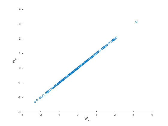
  • We plot the values in the transformed space \(M, N\) for one dimension:

• Why did we get perfect correlation?

  • See the following paper .

  • Previous work (Hardoon et al. \(2004\)) shows that using kernel CCA with no regularization will be likely to produce perfect correlations between the two views. These correlations can therefore fail to distinguish between spurious features and those that capture the underlying semantics. Thus it is important to use regularization to come up with correlation between meaningful features.

• Then we found a different package implementing CCA which allowed us to use regularization on regular CCA, since Matlab did not have regularization parameters

  • Here we avoided running on the SVD version of fMRI and EEG, and just ran on the full matrices. We got much better looking results here since we did not overfit as much with correlation, and got correlation \(0.9448\).

  • We also plotted the covariance for one of the dimensions (\(M, N\) for one dimension):

  • This package took as input the kernel matrices, so in the future we can explore using kernel CCA with regularization for non-linear kernels.

• Bayesian CCA Model

  • Input for fitting: EEG and fMRI

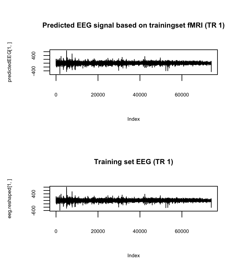
  • We had a Gaussian latent variable \(z\) (chose dimension \(100\)), where we assumed that the mean of each EEG value \((2000\times 37)\times 1\) vector is a linear projection \(A\) of \(z\), and the mean of each fMRI value \((32\times 64\times 64)\times 1\) vector is a linear projection \(B\) of \(z\). We also predicted covariance matrices for the values of EEG and fMRI time steps. Then, have trained the generative model with Bayesian CCA, we predicted the whole EEG time series \((2000\times 37)\times 170\). (which was an input).

  • 

  • This EEG prediction is nearly identical to the EEG input, so this makes sense! (average correlation of prediction vs. true EEG is \(0.97\)).

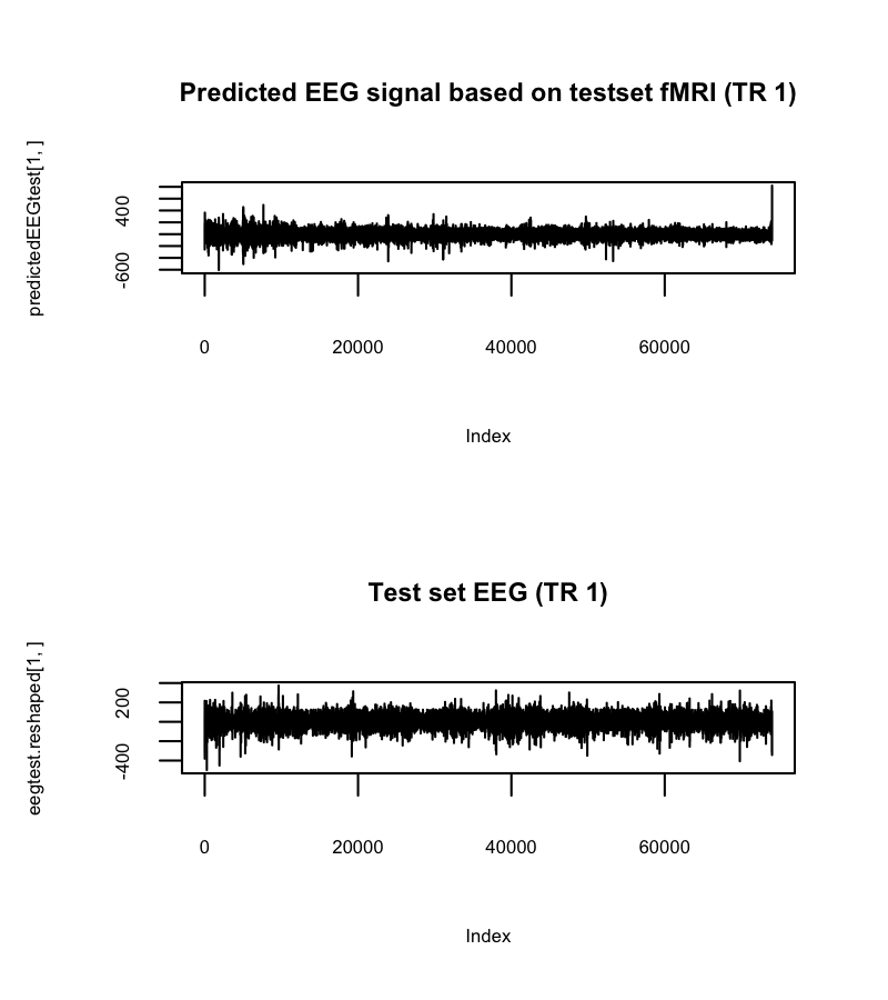
  • Then we used our trained EEG model and used it to predict the EEG for another task run (same task). (given fMRI for the other task run, we predict EEG). We also visualize it.

  • 

  • On the different task, the predicted EEG and the true EEG has roughly \(0\) correlation! This is terrible and thus the approach seems flawed.

  • However, note that the correlation of the prediction of the test set EEG (subject \(1\) task \(1\) run \(2\)) and the prediction of the training set EEG (subject \(1\) task \(1\) run \(1\)) had correlation of \(0.42\), meaning that the algorithm did not merely memorize the data from the test set.

  • One thing we could do is improve our training procedure (we only trained for \(10\) iterations in interest of time) - we can train for more iterations and see how well it does.

• Next steps: Use Sparse CCA

  • The Sparse CCA paper

  • Sparse CCA code

  • We tried running sparse CCA with some preliminal results, but we will go into more detail later!

• MEG Data

  • We received the fMRI-MEG data for the object detection task this morning! We plan to analyze this data in a similar fashion and see if we can come up with a similar model structure here.

Background Survey

Our goals (\(X\) = EEG, \(Y\) = fMRI)

• find \(f(X) = Y\)
• find \(f(Y) = X\)
• find a low-dimensional mapping \(f(X, Y) \to X’\) where \(X’\) is low-dim EEG
• find a low-dimensional mapping \(f(X, Y) \to Y’\) where \(Y’\) is low-dim fMRI
• have a probabilistic generative model for \(X’\) and \(Y’\) (perhaps used in \(f\)

Assessing the quality of \(X’, Y’\)

• Supervised (predictive) tests
  • predict EEG signal from fMRI (accuracy)
  • predict fMRI signal from EEG (accuracy)
  • predict modality of signal type (auditory or visual) from oddball data
  • predict oddball signal on both auditory and visual data
  • how well does generative model do for covarying with \(X’\) and \(Y’\)?
• Unsupervised tests
  • analyze covariation of low-dimensional signal with high-dimensional signals
  • comment on correlations
  • goodness of generative model: compare with actual data (standard statistics)

Prior Methods and Approaches

Generally, prior approaches either use both fMRI and EEG in conjunction as separate information sources to verify neuroscientific claims, or map them into the same space with joint-ICA or CCA, potentially fitting a basic linear model with features from EEG to fMRI.

Data Analysis Approaches

• General Overview of Approaches

  • fMRI-informed EEG aims to localize the source of the EEG data by using fMRI to construct brain model EEG-informed fMRI: extract specific EEG feature, assuming its fluctuations over time covaries

  • Neurogenerative modeling: similar to EEG-source modeling; inverse modeling based on the simulation of biophysical processes (known from neuroscience) involved in generating EEG and fMRI signals.

  • Data fusion [What we are most interested in]: Using supervised or unsupervised machine learning algorithms to combine multimodal datasets

• Late fusion methods [Multivariate Machine Learning Methods for Fusing Multimodal Functional Neuroimaging Data - Biessmann et al]

  • Supervised methods (either using an external target signal or asymmetric fusion where features from one modality are used as labels/regressors to extract factors from another modality) vs unsupervised (relying on data stats)

  • Unsupervised: PCA (maximal variance, decorrelated components), ICA (statistically independent components; temporal ICA for EEG, spatial for fMRI) Studies have found PCA works as well as ICA, with less to tune.

  • Supervised: regression and classification using external target signal (e.g stimulus type/intensity/latency, response time, artifactual information - linear regression, LDA) or using band-power features.

• Early fusion methods [Multivariate Machine Learning Methods for Fusing Multimodal Functional Neuroimaging Data - Biessmann et al]: First forming a feature set from each dataset followed by exploration of connections among the features.

  • Multimodal ICA: joint ICA (features from multiple modalities simply concatenated); parallel ICA (a user specified similarity relation between components from the different modalities is optimised simultaneously with modality-specific un-mixing matrices); linked ICA (Bayesian)

  • CCA and PLS: find the transformations for each modality that maximise the correlation between the time courses of the extracted components. Partial least squares aims to find maximally covarying components, CCA finds maximally correlating components. Relaxes independent component assumption of jICA, does not constrain component activation patterns to be the same for both modalities.

  • mSPoC: co-modulation between component power and a scalar target variable z can be modeled using the SPoC objective function; in multimodal case, assume the target function z is the time-course of a component that is to be extracted from the other modality

Previous Results (Successes and Failures)

• EEG + fMRI (Walz et. al., 2013) on the Oddball dataset (our dataset)

  • EEG data \(\to\) training linear classifier to maximally discriminate standard and target trials \(\to\) create an EEG regressor out of demeaned classifier output (convolved with HRF) \(\to\) use the EEG regressor (and other event or response time related regressors) to fit a linear model to fMRI data \(\to\) comment on the correlation based on the coefficients (positive or negative, p-values). Also, they manually looked at fMRI images at TRs with high degree of correlation with the regressors.

  • How did they validate their performance?

    • They use the p-values of the coefficients to filter out correlates that are insignificant
    • Qualitative images and ‘eyeballing it’-based analyses; comparing to previous known work to demonstrate that the data validates a neuroscientific model
    • P1 response, P300 response, etc (Calhoun paper)
• MEG + fMRI (Cichy et. al., 2014)
  • Used MEG and fMRI data to analyze the hierarchy of the visual pathway in the brain applied to object recognition (i.e., At what stage of visual processing does the brain disambiguate between human and non-human faces? How about man-made versus natural objects?)
  • How did they validate their performance?
    • Made plots of predictive power based on (MEG signal at each time point) over time, notice (with eyes) that peaks correspond to neuroscientifically-known time points in the visual process
    • Correlate the human fMRI with a monkey fMRI and report correlations for the same task
    • Generally, look at covariance plots and describe statistics for the time-points which are neuroscientifically known to be relevant for the neural visual processing pipeline
• mCCA vs jICA (2008)
  • Canonical Correlation Analysis for Feature-Based Fusion of Biomedical Imaging Modalities and Its Application to Detection of Associative Networks in Schizophrenia - Correa et al
  • Uses CCA to make inferences about brain activity in schizophrenia (found patients with schizophrenia showing more functional activity in motor areas and less activity in temporal areas associated with less gray matter as compared to healthy controls), general brain function (fMRI and EEG data collected for an auditory oddball task reveal associations of the temporal and motor areas with the N2 and P3 peaks)
  • The multimodal CCA (mCCA) method, we introduce is based on a linear mixing model in which each feature dataset is decomposed into a set of components (such as spatial areas for fMRI/sMRI or temporal segments for EEG), which have varying levels of activations for different subjects. A pair of components, one from each modality, are linked if they modulate similarly across subjects.
  • How did they validate their performance?
    • Generated a simulated fMRI like set of components and an ERP-like set of components and mix each set with a different set of modulation profiles to obtain two sets of mixtures. The modulation profiles are chosen from a random normal distribution. The profiles are kept orthogonal within each set. Connections between the two modalities are simulated by generating correlation between profile pairs formed across modalities
  • Compares mCCA with jICA:
    • 
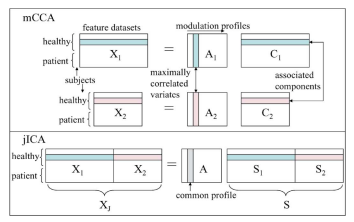
    • jICA examines the common connection between independent networks in both modalities while mCCA allows for common as well as distinct components and describes the level of connection between the two modalities
    • jICA model requires the two datasets to be normalized before being entered into a joint analysis underlying assumption of made in jICA is more reasonable when fusing information from two datasets that originate from the same modality
    • independence assumption in jICA; but utilizes higher order statistical information
    • mCCA jointly analyzes the two modalities to fuse information without giving preference to either modality; does not assume a common mixing matrix and does not require the data to be preprocessed to ensure equal contribution from both modalities
    • mCCA assumes that the components are linearly mixed across subjects
• Deligianni et. al (2014): Relating resting-state fMRI and EEG whole-brain connectomes across frequency bands
  • Apply sparse-CCA with randomized Lasso to fMRI-connectome and EEG-connectome for resting-state data (i.e., no supervised task) to identify the connections which provide most signal
  • Analyze the distance between precision matrices of the Hilbert envelopes (for fMRI and EEG)
    • Assuming brain activity patterns are described by a Gaussian multidimensional stationary process, the covariance matrix fully characterizes the statistical dependencies among the underlying signals
  • They estimate prediction error via cross-validation for a function \( f(\Omega^F) \approx \Omega^E \)

Our Points of Novelty

• Most people don’t think the fMRI and EEG data is low-dimensional, and thus don’t go beyond vanilla approaches to find structure, with the exception of the Deligianni paper

• We can take advantage of the structure over time and space in fMRI and EEG data to reduce dimension and induce sparsity

• Most people do not focus on coming up with generative models for fMRI / EEG data (except for 4 groups or so: John Cunningham, Jonathan Pillow and two others).

• We can go beyond Gaussian process assumptions to potentially create a more realistic view of the signals

• Use information-theoretic features in addition to typical neuroscientific features; validate results of the Assecondi paper

Details of Our Approach

• What methods will you use to analyze these data?
  • How will features be represented?
    • as vectors in space and time
      • vector in space varying over time (fMRI representations are sparse)
      • vector in time varying over space (EEG representations are sparse)
    • we can leverage a variety of dimension reduction approaches (both linear and non-linear)
    • use mutual information \(\mathcal{I}\) between points as a feature
    • use entropy \(H\) as a feature
  • What probabilistic models can we use to capture important signal in these data?
    • GLM (what everyone uses) with sparse features (after dimension reduction - sparse PCA?)
    • sparse CCA (following Deligianni et. al. but applied to predictive models)
    • Generative model with general non-gaussian distributions (for instance, fourth moment not \(3\)
      • Common underlying sources generate EEG and fMRI by mixing with EEG-specific noise sources and fMRI-specific noise sources
    • Can apply similar approach from Cichy et. al (2014)
      • Use machine learning classifier as a proxy for the predictive power of EEG signal at a given state
  • Information-theoretic models
    • Most people using simultaneous EEG-fMRI rely on fitting a general linear model (in most cases, this is just a plain linear model with a linear mixing matrix etc) to describe the correlation between EEG and fMRI data.
    • Thus most people only focus on linear correlation
    • Our alternative: Use mutual information and entropy to measure correlation, since these incorporate higher order correlations present in the data
    • Potential drawback: need high quality estimate of underlying probability distribution EEG/fMRI features are usually modeled as Gaussian - this assumption is way too broad
    • We can use different bias correction techniques based on number of samples, amount of correlation, and binning strategy.
• What assumptions are made about the data in the model (explicit and implicit)?
  • There is a high degree of correlation between EEG and fMRI data
  • Sparsity in the components (namely, that the thought signal lives in a much lower dimension, particularly true for the oddball task)
• What will you do if those violated assumptions hurt performance?
  • Add regularization
  • Change model assumptions
• How will you fit the model to the data? Will this be computationally tractable?
  • CCA with regularization to induce sparsity in components.
  • Variational inference (for fitting generative model)
• How will you validate performance?
  • We have some supervised tasks (as mentioned before); here, we can just assess predictive error
  • We can also plot the data in interesting formats (over time, in low dimension, etc.) to assess qualitatively if the results are meaningful
  • We can compare our results to neuroscientific literature to see if our models hold up to previously known results
• Is it feasible to compare our methods against other methods and to compare models?
  • Yes, it is very feasible; we can compare with normal joint-ICA and non-sparse CCA
• Do reasonable implementations of the methods exist?
  • sparse-CCA has a reasonable implementation
  • variational inference fitting will depend on the specific assumptions we make about the priors
    • David Blei’s group at Columbia is working on message-passing algorithms for plug-and-chug variational inference

Links

• Multivariate Machine Learning Methods for Fusing Multimodal Functional Neuroimaging Data [Dähne et. al., 2015]
• Canonical Correlation Analysis for Feature-Based Fusion of Biomedical Imaging Modalities and Its Application to Detection of Associative Networks in Schizophrenia [Correa et. al., 2008]
• Relating resting-state fMRI and EEG whole-brain connectomes across frequency bands [Deligianni et. al, 2014]
• Simultaneous EEG-fMRI reveals temporal evolution of coupling between supramodal cortical attention networks and the brainstem [Walz et. al., 2013]
• Neuronal chronometry of target detection: fusion of hemodynamic and event-related potential data [Calhoun et. al., 2006]
• Resolving human object recognition in space and time [Cichy et. al., 2014]
• Methods for simultaneous EEG-fMRI: an introductory review [Huster. et. al, 2012]
• Reliability of Information-Based Integration of EEG and fMRI Data: A Simulation Study [Assecondi et. al., 2015]

Overview

Goals

We are interested in exploring the relationships between different measurements of brain activity, namely, fMRI, MEG, and EEG. fMRI data is based on a time series of BOLD responses and takes the form of a 4-vector with high spatial resolution, but low temporal resolution. On the other hand, both MEG (recordings of magnetic fields induced by electrical currents in the brain) and EEG (recording voltage fluctuations due to ion movement inside neurons) data have high temporal resolution, but less spatial resolution. Therefore, the primary question we ask for our project is: Can we utilize fMRI and (EEG or MEG) data, recorded simultaneously on a set of subjects performing some task, to jointly create a new signal that is able to retain both spatial and temporal resolution from the inputs to achieve a higher resolution on both axes? If we take \(X\) to be EEG-space and \(Y\) to be fMRI space, we essentially wish to find two functions

such that \(X’\) and \(Y’\) are better representations of the underlying information in the brain data.

We would also like to validate our multimodal representation with results on tasks like predicting the object a person is looking at, in order to demonstrate an improvement over the unimodal representations.

The Dataset

We are currently using the Auditory and Visual Oddball EEG-fMRI dataset, available for download at the following link . The complete description of the data is available at the provided link. We summarize the main points here:

• 17 healthy subjects performed separate but analogous auditory and visual oddball tasks (interleaved) while simultaneous EEG-fMRI was recorded.

• The Oddball experiment paradigm: There were 3 runs each of separate auditory and visual tasks. Each run consisted of 125 total stimuli (each 200 ms): 20% were target stimuli (requiring a button response) and 80% were standard stimuli (to be ignored). The first two stimuli in the time course are constrained to be standard stimuli. The inter-trial interval is assumed to be uniformly distributed over 2-3 seconds.

  • Task 1 (Auditory): The target stimulus was a broadband “laser gun” sound, and the standard stimulus was a 390 Hz tone.

  • Task 2 (Visual): The target stimulus was large red circle on isoluminant grey background at a 3.45 degree visual angle, and the standard stimulus was a small green circle on isoluminant grey background at a 1.15 degree visual angle.

• The EEG data was collected at a 1000 Hz sampling rate across 49 channels. The start of the scanning was triggered by the fMRI scan start. The EEG clock was synced with the scanner clock on each TR (repetition time).

• The BOLD fMRI Data was an EPI sequence with 170 TRs per run, with 2 sec TR and 25 ms TE (echo time). There are 32 slices, and no slice gap. The spatial resolution is 3mm x 3mm x 4mm with AC-PC alignment.

Related Papers

• Prestimulus EEG alpha oscillations modulate task-related fMRI BOLD responses to auditory stimuli [Walz et. al, 2015]

• Simultaneous EEG-fMRI reveals a temporal cascade of task-related and default-mode activations during a simple target detection task [Walz et. al, 2014]

• Fast bootstrapping and permutation testing for assessing reproducibility and interpretability of multivariate fMRI decoding models [Conroy et. al, 2013]

• Simultaneous EEG-fMRI reveals temporal evolution of coupling between supramodal cortical attention networks and the brainstem [Walz et. al, 2013]

• Joint independent component analysis for simultaneous EEG-fMRI: principle and simulation [Moosmann et. al, 2007]

• Electrophysiological correlates of the BOLD signal for EEG-informed fMRI [Murta et. al., 2015]

• Data-driven analysis of simultaneous EEG/fMRI using an ICA approach [Schmüser et. al., 2014]

• Reliability of information-based integration of EEG and fMRI data: a simulation study [Assecondi et. al, 2014]

Preliminary Analysis

Exploratory Analysis of the EEG Data

Below is the raw EEG data from the experiment, where each horizontal time series is an EEG-source with a few exceptions. The first 43 channels are EEG electrodes, channel 44 and 45 are EOG (eye movement), channel 46 and 47 is ECG (heart), and channel 48 and 49 are the stimulus and the behavioral response event markers, respectively.

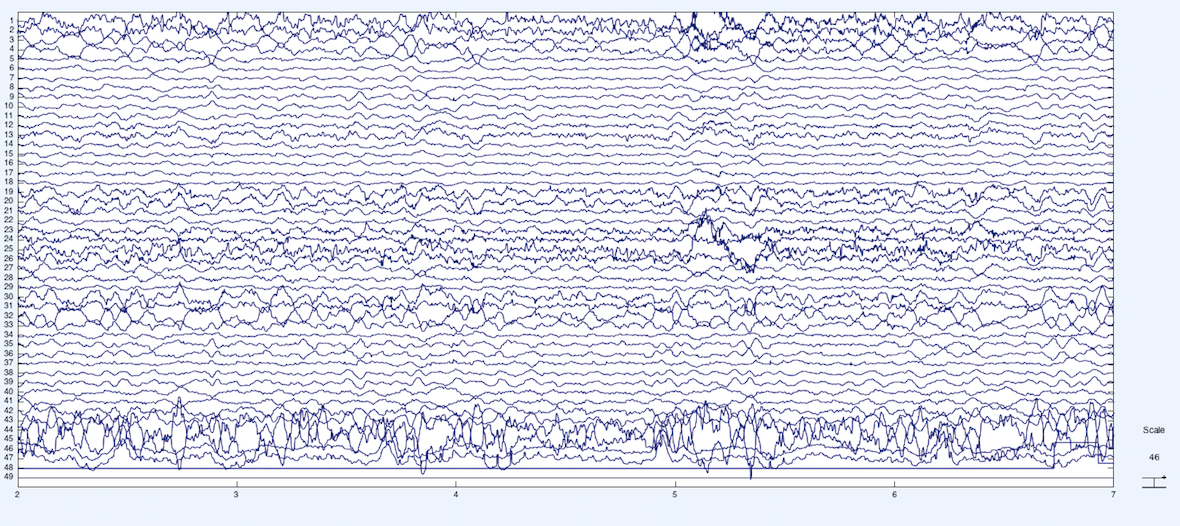
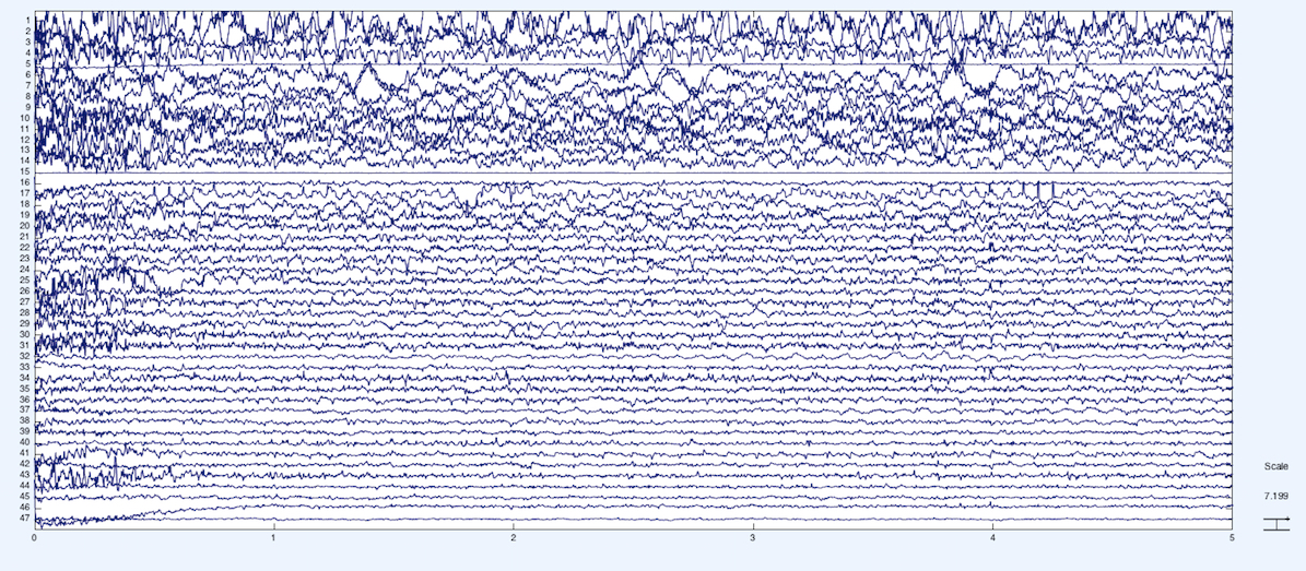
We plot the same data after performing Independent Components Analysis (ICA) along the time series. We can see that the first few channels of EEG explain a lot of the variance.

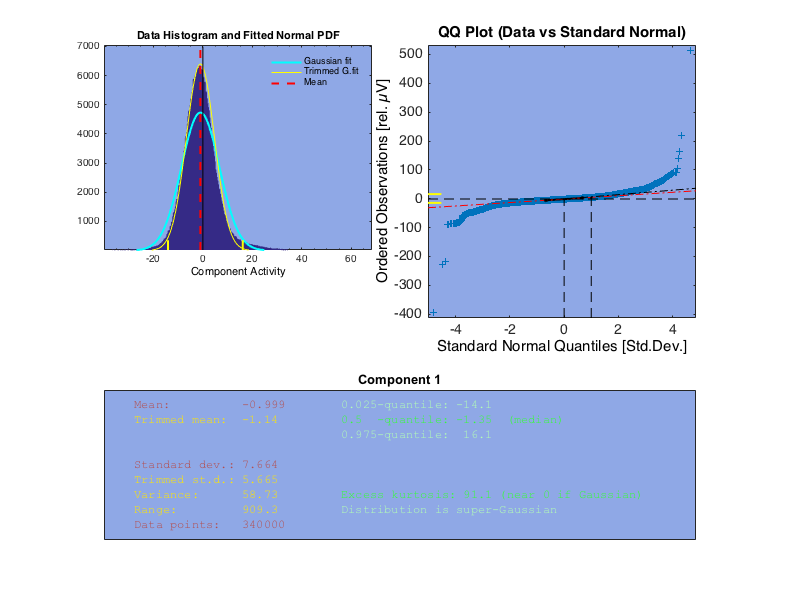
Here we examine the first component after ICA is performed on the EEG data. The first plot is of the variation in EEG response values. We see that for the first component, the response is roughly Gaussian. This approximation roughly holds across the other components, though the kurtosis varies.

Here we plot a correlation matrix of the EEG channels for the auditory task. The value of entry (i, j) is the covariance between two EEG channels summed over time. There appears to be an interesting block structure, suggesting that some channels are highly correlated with each other, while others are not. This correlation matrix allows us to check how we might reduce dimension later on.

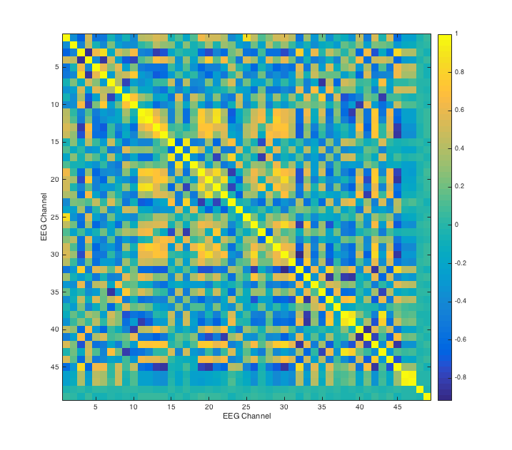
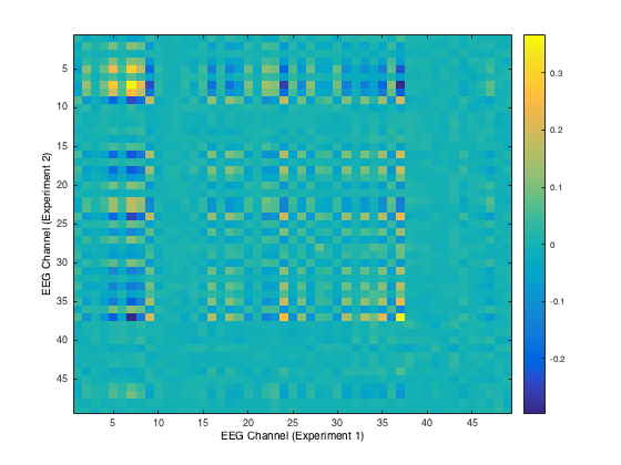
Here, we plot a correlation matrix of the EEG channels across both the auditory and visual tasks for the first run in both tasks. We take covariances by summing over time for each channel pair, where one channel is the EEG response over auditory and the other channel is the EEG response over visual. This correlation matrix allows us to notice that across experiments, most of the EEG channels are not correlated with each other. Perhaps the channels that remain correlated signify more information about responses to stimuli (of various types) than the others.

Exploratory Analysis of the fMRI Data

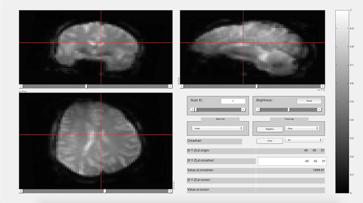
Here we have a nice visualization of the fMRI data. Notice that it looks like a brain!

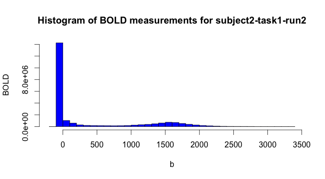
Then we simply binned the values of the fMRI data to get a general idea of what responses looked like. Note that a lot of the fMRI values are 0. When subsampling to plot covariances and so on, we drew voxels from the non-zero space.

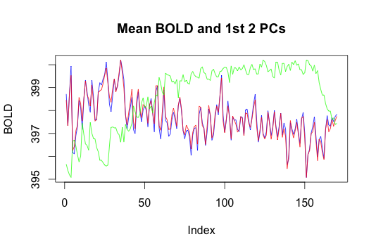
Here we plotted the mean BOLD response and the first two principal components. We performed PCA to reduce the voxel space dimension on a single subject’s fMRI data for task 1, run 2. The resulting components are therefore time vectors: The horizontal axis of the plot is time, and the vertical axis is response. The color scheme is as follows: blue is the mean, red is the first principal component and green is the second principal component. The first PC appears very close to the mean and it appears to explain 99% of the variance. This result is not what we expected, and possibly suggests that applying PCA directly may not be the best way to reduce the dimension of the data, due to the highly non-linear variation of the BOLD values of fMRI voxels. Thus we may explore nonlinear dimension reduction approaches like Local Linear Embedding or Isomap. Since we may be looking for signal in a very small percentage of the voxels, another interpretation of the result may be that our confusing results are due to the strong effect of noise (i.e. the voxels we are not interested in) on the results of PCA in high dimension. Thus, the 99% explained by the first principal component may only be explaining variance in voxels we are not interested in (also recall that from the histogram, most of the voxels are 0).

Here we plot a correlation matrix for each TR: At each time step, we calculate covariance by summing over voxels.

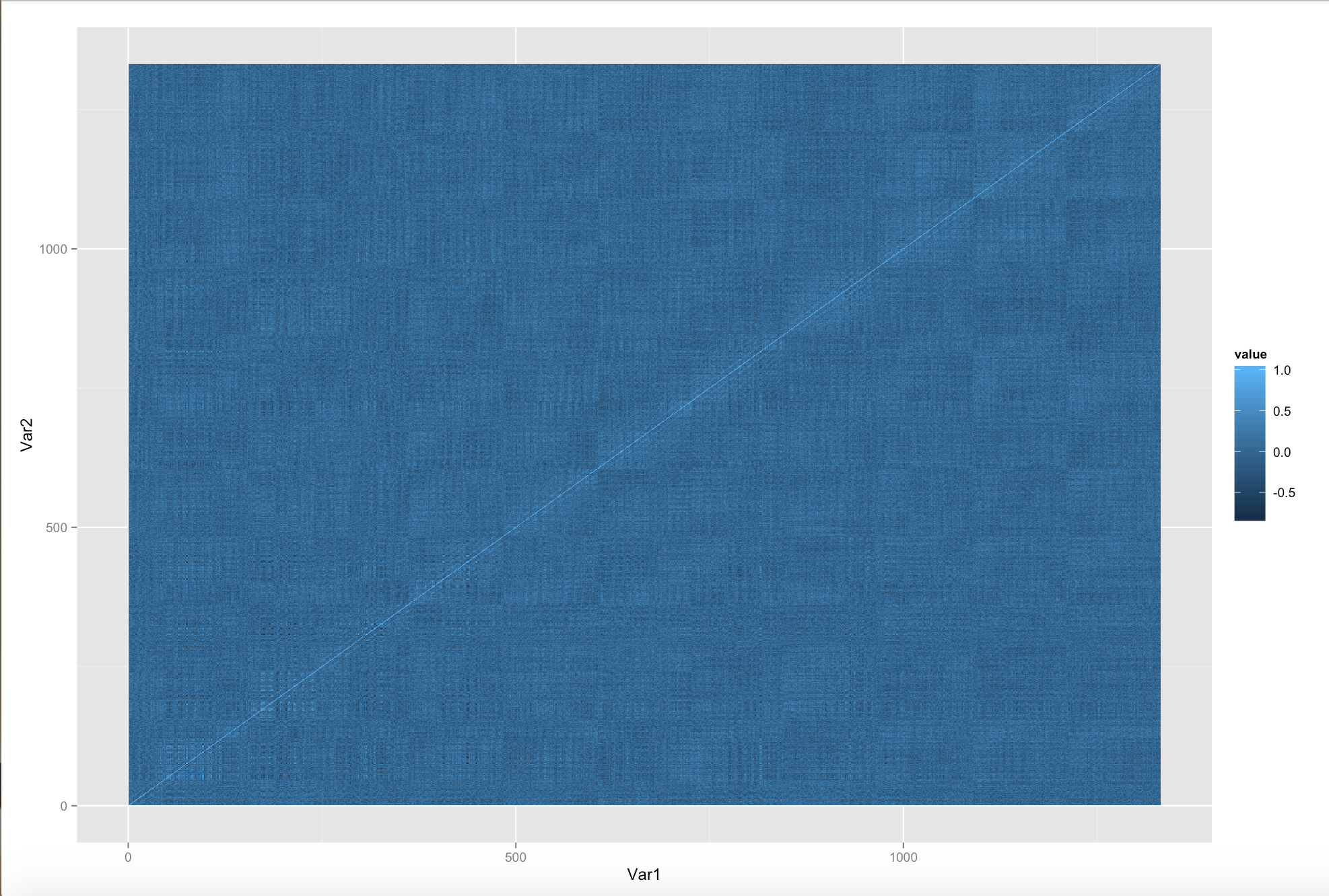
Here we plot a correlation matrix for a subset of the voxels from the center of brain. Here, for each voxel pair, we calculate covariance by summing over time.

Future Directions

• Investigate cross-correlation of the EEG and fMRI data at full scale. We did not implement this cross-modality analysis since we felt it would be less meaningful if we only sampled a small portion of the fMRI voxels while comparing to EEG sources, as running covariance calculations for large number of voxels crashed the software we were using to generate them (which is why we display a correlation matrix with only a small number of voxels on each axis). We will use a cluster to investigate the full correlation matrix of the fMRI voxel data, as well as the correlation between the EEG and fMRI data.

• Apply more dimension reduction methods and plot time courses in two dimensions to see if any patterns arise.

• Apply community detection analysis to the fMRI data.